Richard B. Johnson
Foreword
When I started out in the electronics industry I had been trained in RF technology and I designed equipment that used vacuum tubes! Somewhere along the way, the tubes went away, being replaced with transistors and microprocessors. My work moved with the technology so nowadays most of it involves software. This is my attempt to share some newer technology with many older engineers who might be afraid to ask. This is about the FFT, windowing, and software to make a virtual spectrum analyzer. Using the included source-code, both engineers and technicians can make many interesting projects using their PCs.
Examining the FFT
If you take a buffer full of data, perhaps something you got from the audio board on your PC or extracted from a “wave” file, and ran a FFT [5] on it, it would have many spurious responses, be too wide for a useful display, and not look very much like what one would expect from a spectrum analyzer. Here is an example of a pure sine-wave at 32 Hz displayed without a window.
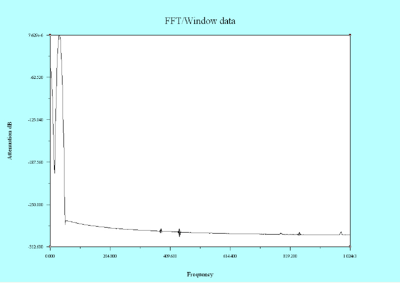 |
In fact, if you made a mathematically perfect tone, with no distortion, the FFT would show responses that you know are not correct. Analyzing a simple waveform, like a pure sine wave, causes its Fourier transform to have non-zero values (commonly called leakage) at frequencies other than the fundamental. It tends to be worst (highest) near the fundamental frequency, and lesser at frequencies farthest from it. If there are two sinusoids with different frequencies leakage can interfere with the ability to distinguish them spectrally. If their frequencies are dissimilar the leakage interferes when one sinusoid is much smaller in amplitude than the other. What is happening?
The problem is that the FFT expects data to be continuous. Since buffers full of data are not continuous because they have a start and stop (beginning and ending), they are not displayed correctly unless they are processed first. Such processing is called windowing and there are many different kinds of windows.[3] If you were to slowly increase the level of the data in the buffer from zero to its normal level, so that the data is “turned on” very slowly, any disturbances and the sideband signals they cause are moved in close to the fundamental frequency bin. This will tend to make them disappear. Of course, you would have to turn the data off very slowly as well.
For instance, if you had a resolution of 10 Hz on your display, and it took one-tenth of a second to smoothly go from zero to maximum amplitude, then you would see the disturbance from zero to 10 Hz, but there would not be many artifacts displaced higher in frequency than 10 Hz from the fundamental. The idea of a window is to move any artifacts generated by the discontinuous data close to the fundamental frequency where they are inconsequential.
There are additional problems associated with sampled data systems. All the bins are modulated with the sample-rate so that to the observer, an individual spectral component appears to consist of a large number of sideband components, plus if the fundamental frequency of the signal being observed becomes synchronous with the sample rate, it may disappear altogether.
Typically a window’s components start at 0 and increase in magnitude to some maximum value. The function that generates this window may have several names. When windowing a FFT every element in the array of data is multiplied by an element at the same location (offset) in the window. Such a data buffer containing a window is called a kernel. One that is easy to understand is the raised cosine, sometimes called the “Hanning” window. It is shown here.[2]
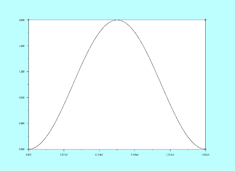 |
This graph has 16384 bins or samples, the same number of samples that our signal to be analyzed has. Its amplitude goes from 0 to 2. However, its shape is that of an elevated cosine. The maximum amplitude goes to 2 so that are area under the curve is exactly 1. If this was not the case, voltage measurements from the bins (samples) would be incorrect. If the window is only used for a spectrographic view, such scaling is not necessary. In the sample code, the raised cosine window is used for some voltage measurements so it needs to preserve the area.
Here is another window called the “Hamming” window. It uses a “Hamming” function to generate it. Its values range from not quite 0 to 1. It has the same number of samples as the raised cosine window.
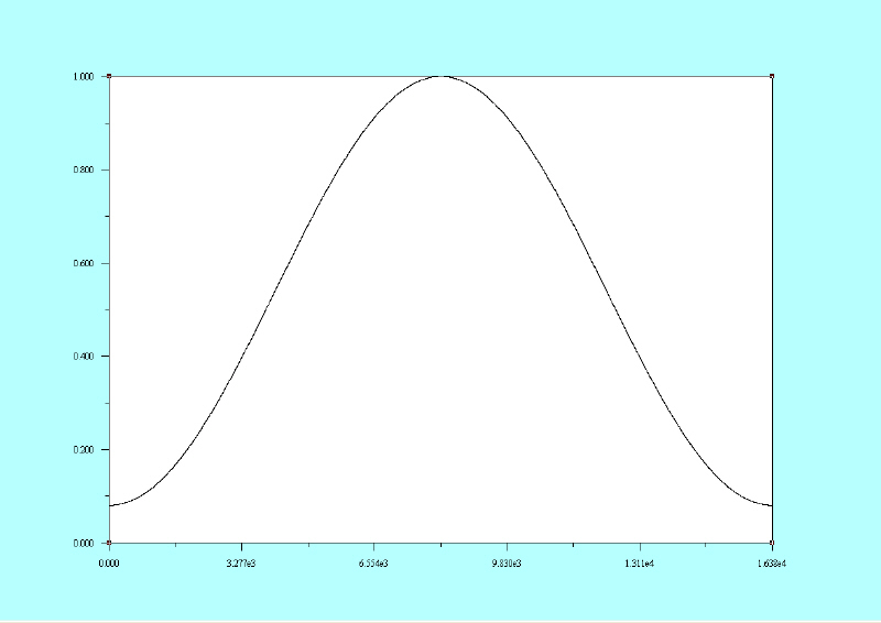 |
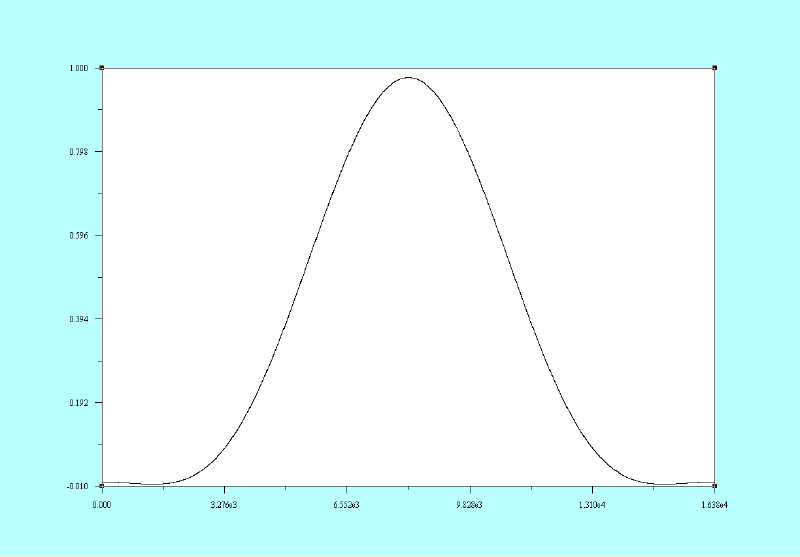
Notice that its shape is somewhat different than the raised cosine window. The following is the “Blackman-Harris” window and it uses a function by the same name for its generation.
 |
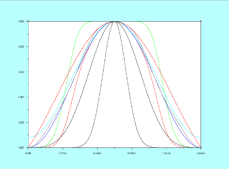
Each of these windows has a particular advantage and also some disadvantages when viewing a spectrographic image. The referenced software contains many windows with the software functions necessary to generate them.[1]
This chart graphs the window functions included with the software. When making a virtual instrument it may be advantageous to allow an operator to select many such windowing functions.
 |
By selecting the proper window, one can obtain a very good approximation of a spectrum analyzer display. Here is an image obtained from the data used in the first example at the top of this page by using the Blackman-Harris window.
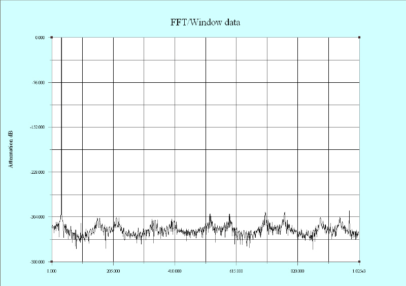 |
This image was obtained from a “perfect” software-generated sine-wave at 32 Hz. Any artifacts are caused by round-off errors in the floating-point routines. These artifacts are far below any spurious responses expected in real signals. All of these utilities are included in the referenced software.[1]
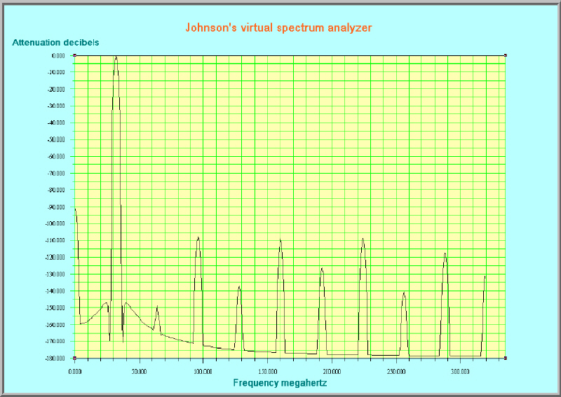
Here is an example of a virtual spectrum analyzer display using real data from a signal generator, captured with a 1 GHz digitizer. In this case the noise and spurious responses are about 100 dB below the carrier.
 |
The software produces data files as output from its examples. The images shown on this Webpage were created from those data files using “Presto.” Its source code is referenced below as well.[4]
References
1. Source code for Johnson’s free signal processing library
2. Common window functions
3. MIT paper on FFT/DFT windows
4. Source code for “Presto” imaging software
5. The Fast Fourier Transform (FFT)
External links
Author’s website
Notes
This article may be freely copied or referenced. No copyright protection is claimed. The underlying HTML code is also in the public domain.